1. 简介

- 最小二乘在科研与实践中的重要性

普通最小二乘法（Ordinary Least Squares, OLS）通常用于回归问题，而非直接用于分类问题。不过，在某些情况下，最小二乘法可以被改编用于分类任务，例如通过设定阈值将连续输出转化为离散类别，或者在特定假设下（如线性判别分析的背景下）将其与分类联系起来。

2. 论文证明：最小二乘的理论基础

- 如何通过最小二乘支撑论文的论点和假设

这里提供了基于公理化证明方法，

截图如下：

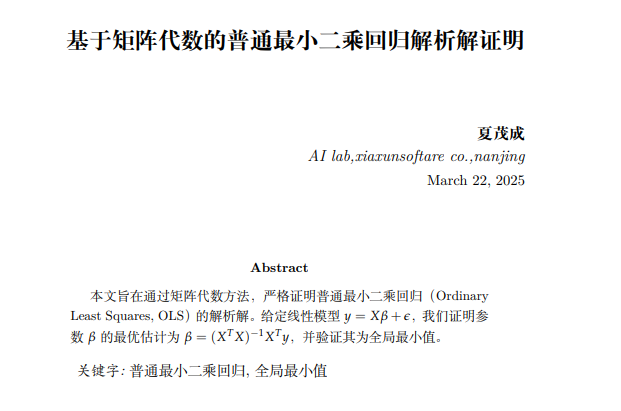
整体证明，有兴趣的链接直达：不干兴趣的直接跳过。

基于矩阵代数的普通最小二乘回归解析解证明.pdf

- 实例分析：论文中最小二乘的典型案例

限于篇幅，如下采用了官文。

3.代码分析：最小二乘的工具与技术

- 最小二乘中常用的编程语言python和工具基础包

这里直接使用了科学包，

- 如何编写高效、可靠的最小二乘代码

为了验证我们之前所述的思想：我们给出简单的实现：

以下是使用 Python 从零开始实现 Scikit-learn 风格的最小二乘线性回归算法的完整代码：

import numpy as np
class LinearRegression:
    def __init__(self, fit_intercept=True):
        self.fit_intercept = fit_intercept
        self.coef_ = None
        self.intercept_ = None
    def fit(self, X, y):
        # 将输入转换为 numpy 数组
        X = np.array(X)
        y = np.array(y)
        # 确保 y 是二维数组 (n_samples, m_outputs)
        if y.ndim == 1:
            y = y.reshape(-1, 1)
        # 添加偏置项（截距项）
        if self.fit_intercept:
            ones = np.ones((X.shape[0], 1))
            X = np.hstack((X, ones))
        # 计算系数
        X_T = X.T
        X_T_X = X_T.dot(X)
        X_T_X_inv = np.linalg.pinv(X_T_X)
        X_T_y = X_T.dot(y)
        w = X_T_X_inv.dot(X_T_y)
        # 分割系数和截距项
        if self.fit_intercept:
            self.coef_ = w[:-1, :]
            self.intercept_ = w[-1:, :]
        else:
            self.coef_ = w
            self.intercept_ = np.zeros((1, y.shape[1]))
        # 如果是单输出，调整形状为 1D 数组和标量
        if y.shape[1] == 1:
            self.coef_ = self.coef_.ravel()
            self.intercept_ = self.intercept_.ravel()[0]
        return self
    def predict(self, X):
        X = np.array(X)
        if self.fit_intercept:
            return X.dot(self.coef_) + self.intercept_
        else:
            return X.dot(self.coef_)
# 测试代码
if __name__ == "__main__":
    # 测试数据 1: 无截距项
    X1 = np.array([[1], [2], [3]])
    y1 = np.array([2, 4, 6])
    
    model1 = LinearRegression(fit_intercept=False)
    model1.fit(X1, y1)
    print("Test 1:")
    print("Coefficients:", model1.coef_)
    print("Intercept:", model1.intercept_)
    print("Prediction for 4:", model1.predict(), end="\n\n")
    # 测试数据 2: 有截距项
    X2 = np.array([[1], [2], [3]])
    y2 = np.array([3, 5, 7])
    
    model2 = LinearRegression()
    model2.fit(X2, y2)
    print("Test 2:")
    print("Coefficients:", model2.coef_)
    print("Intercept:", model2.intercept_)
    print("Prediction for 4:", model2.predict(), end="\n\n")
    # 测试数据 3: 多特征
    X3 = np.array([[1, 2], [2, 4], [3, 6]])
    y3 = np.array([3, 5, 7])
    
    model3 = LinearRegression()
    model3.fit(X3, y3)
    print("Test 3:")
    print("Coefficients:", model3.coef_)
    print("Intercept:", model3.intercept_)
    print("Prediction for [4, 8]:", model3.predict([[4, 8]]))

这个实现完整展示了最小二乘法的核心原理，同时保持了与 Scikit-learn 相似的接口设计，可以直接用于简单的回归任务。

- 案例分析：使用代码进行数据清洗、可视化和建模的过程

4. 实验验证：最小二乘的实践意义

为了方面，下文将采用统一的。我们熟知的API进行设计：

- 实验设计在最小二乘中的重要性

- 如何设计和执行有效的数据实验

为此，我们使用糖尿病数据集中的单个功能，并尝试使用该线性模型来预测糖尿病的进展。因此，我们加载糖尿病数据集并将其分为训练和测试集。

然后，我们将模型安装在训练集上，并在测试集上评估其性能，并最终可视化测试集中的结果。

"""
==============================
Ordinary Least Squares Example
==============================
This example shows how to use the ordinary least squares (OLS) model
called :class:`~sklearn.linear_model.LinearRegression` in scikit-learn.
For this purpose, we use a single feature from the diabetes dataset and try to
predict the diabetes progression using this linear model. We therefore load the
diabetes dataset and split it into training and test sets.
Then, we fit the model on the training set and evaluate its performance on the test
set and finally visualize the results on the test set.
"""
# Authors: The scikit-learn developers
# SPDX-License-Identifier: BSD-3-Clause
# %%
# Data Loading and Preparation
# ----------------------------
#
# Load the diabetes dataset. For simplicity, we only keep a single feature in the data.
# Then, we split the data and target into training and test sets.
from sklearn.datasets import load_diabetes
from sklearn.model_selection import train_test_split
X, y = load_diabetes(return_X_y=True)
X = X[:, [2]]  # Use only one feature
X_train, X_test, y_train, y_test = train_test_split(X, y, test_size=20, shuffle=False)
# %%
# Linear regression model
# -----------------------
#
# We create a linear regression model and fit it on the training data. Note that by
# default, an intercept is added to the model. We can control this behavior by setting
# the `fit_intercept` parameter.
from sklearn.linear_model import LinearRegression
regressor = LinearRegression().fit(X_train, y_train)
# %%
# Model evaluation
# ----------------
#
# We evaluate the model's performance on the test set using the mean squared error
# and the coefficient of determination.
from sklearn.metrics import mean_squared_error, r2_score
y_pred = regressor.predict(X_test)
print(f"Mean squared error: {mean_squared_error(y_test, y_pred):.2f}")
print(f"Coefficient of determination: {r2_score(y_test, y_pred):.2f}")
# %%
# Plotting the results
# --------------------
#
# Finally, we visualize the results on the train and test data.
import matplotlib.pyplot as plt
fig, ax = plt.subplots(ncols=2, figsize=(10, 5), sharex=True, sharey=True)
ax[0].scatter(X_train, y_train, label="Train data points")
ax[0].plot(
    X_train,
    regressor.predict(X_train),
    linewidth=3,
    color="tab:orange",
    label="Model predictions",
)
ax[0].set(xlabel="Feature", ylabel="Target", title="Train set")
ax[0].legend()
ax[1].scatter(X_test, y_test, label="Test data points")
ax[1].plot(X_test, y_pred, linewidth=3, color="tab:orange", label="Model predictions")
ax[1].set(xlabel="Feature", ylabel="Target", title="Test set")
ax[1].legend()
fig.suptitle("Linear Regression")
plt.show()

前置内容不再赘述

- 实例分析：通过实验验证最小二乘结论的可靠性和有效性

如下我们将对应的使用之前的工具来展示：因此，我们获得了给定数据的目标平均值的估计器。

5. 结论

- 最小二乘的综合意义和实践方法

最小二乘法是一种常用的参数估计方法，主要用于寻找数据集与一个线性模型的拟合最优解。其综合意义在于：

1.优化模型拟合度：最小二乘法可以最大程度地减小实际值与预测值之间的误差，使得模型能够更好地拟合数据。

2.推断参数：通过最小二乘法可以计算出线性模型中的参数估计值，从而进行相关的参数推断。

3.评估模型效果：通过检验拟合模型的残差，可以评估最小二乘模型的拟合效果和模型的有效性。

4.处理实际问题：最小二乘法在实际问题中有着广泛的应用，例如经济学领域的回归分析和工程学领域的信号处理等。

实践方法包括以下步骤：

1.建立模型：首先根据实际问题建立线性模型，确定需要估计的参数。

2.构建代价函数：将实际值与模型预测值之间的误差作为代价函数，通常选择残差平方和作为最小化的目标函数。

3.求解最优解：通过最小化代价函数，可以使用数值优化方法如梯度下降法或者通过矩阵求导方法求解最小二乘问题，得到最优解的参数估计值。

4.评估模型：对估计出的模型进行检验，可以计算残差、确定模型的拟合优度、预测效果等。

5.应用模型：最后将建立好的最小二乘模型应用到实际问题中，进行预测、推断或决策。

总的来说，最小二乘法通过寻找最优参数解来优化模型的拟合度，提供了一种实用的方法来处理线性模型的参数估计问题。

- 三大维度的最小二乘相互关联和相辅相成的关系

在统计学中，三大维度的最小二乘法是指在多元线性回归分析中，通过最小化因变量的观测值与回归方程预测值之间的残差平方和来确定回归系数的方法。这三个维度分别是解释变量、因变量和残差。

相互关联的概念指的是在多元线性回归中，解释变量之间存在相关性的情况。如果解释变量之间存在较强的相关性，可能会导致多重共线性问题，影响回归分析的结果和可靠性。

相辅相成是指解释变量与因变量之间的关系是互相促进、相互支持的。在最小二乘法中，我们试图通过解释变量的值来最佳地预测因变量的值，从而建立他们之间的相辅相成的关系。如果回归模型能够很好地描述解释变量和因变量之间的关系，并且残差较小，则说明这种相辅相成的关系是有效的。

因此，在多元线性回归分析中，我们希望解释变量之间不出现过多的关联，同时通过最小二乘法建立解释变量与因变量之间的相辅相成的关系，以获得可靠的回归模型和预测结果。

- 未来最小二乘领域的发展趋势和挑战

未来最小二乘领域的发展趋势和挑战包括以下几个方面：

1.智能化和自动化：未来最小二乘方法的发展将更加注重智能化和自动化。随着大数据和机器学习的发展，未来最小二乘方法将会更多地与深度学习和神经网络相结合，实现数据的自动处理和优化。

2.多模态数据处理：未来最小二乘方法将面临处理多模态数据的挑战，例如同时考虑图像、文本、音频等多种不同类型的数据，需要设计更加复杂和高效的算法来处理这些数据。

3.稀疏数据处理：随着数据的维度不断增加，未来最小二乘方法需要更好地处理稀疏数据，提高模型的泛化能力和鲁棒性。

4.实时性和效率：未来最小二乘方法需要更加注重实时性和效率，特别是在处理大规模数据时，需要设计更快速和有效率的算法以满足实际应用需求。

5.模型解释和可解释性：随着深度学习等黑盒模型的广泛应用，未来最小二乘方法需要更加重视模型解释和可解释性，使模型的结果更容易被理解和接受。

总的来说，未来最小二乘领域的发展将会更加注重智能化、多模态数据处理、稀疏数据处理、实时性和效率以及模型解释和可解释性等方面的挑战。随着科技的不断发展和创新，相信未来最小二乘方法将会更加强大和多样化，为各种领域的应用提供更好的支持。

ITPub博客

探索最小二乘法

最新文章