原文链接： http://tecdat.cn/?p=3071

结构方程模型入门 

介绍

对于熟悉线性回归拟合结构方程模型的分析师来说，在R环境中，拟合结构方程模型涉及学习新的建模语法，新的绘图语法以及通常是新的数据输入方法。然而，拟合结构方程模型可以成为分析师工具箱中的强大工具。

设置 环境

在R中实现SEM有许多不同的包， lavaan软件包为大多数SEM用户提供了全面的功能集，并且具有易于学习的语法来描述SEM模型。要安装 lavaan，我们只需运行：

# Main versioninstall.packages("lavaan")

读入数据

加载lavaan包后，我们需要读入数据集。我们读取方差 - 协方差矩阵并运行路径分析模型。

 mat1 <- matrix(c(1, 0, 0, 0.6, 1, 0, 0.33, 0.63, 1), 3, 3, byrow = TRUE) print(mat1)

##      ILL  IMM DEP## ILL 1.00 0.00   0## IMM 0.60 1.00   0## DEP 0.33 0.63   1

现在我们在我们的环境中命名了一个方差 - 协方差矩阵。

有了这些数据，我们可以构建两种可能的模型

1. 抑郁症（DEP）影响免疫系统（IMM）影响疾病（ILL）
2. IMM影响ILL影响DEP

使用SEM我们可以评估哪个模型最能解释我们在上面的数据中观察到的协方差。拟合模型 lavaan是一个两步过程。首先，我们创建一个文本字符串作为 lavaan模型 。接下来，我们给出 lavaan如何拟合这个模型。

# Specify the model# Give lavaan the command to fit the modelmod1fit <- sem(mod1, sample.cov = mat1, sample.nobs = 500)# Specify model 2 mod2fit <- sem(mod2, sample.cov = mat1, sample.nobs = 500)

现在，我们在环境中为每个模型存储了两个对象。我们有模型字符串和modelfit对象。 summary提供输出：

####   Number of observations                           500####   Estimator                                         ML##   Minimum Function Test Statistic                2.994##   Degrees of freedom                                 1##   P-value (Chi-square)                           0.084#### Parameter estimates:####   Information                                 Expected##   Standard Errors                             Standard####                    Estimate  Std.err  Z-value  P(>|z|)## Regressions:##   ILL ~##     IMM               0.600    0.036   16.771    0.000##   IMM ~##     DEP               0.630    0.035   18.140    0.000#### Variances:##     ILL               0.639    0.040##     IMM               0.602    0.038

####   Number of observations                           500####   Estimator                                         ML##   Minimum Function Test Statistic              198.180##   Degrees of freedom                                 1##   P-value (Chi-square)                           0.000#### Parameter estimates:####   Information                                 Expected##   Standard Errors                             Standard####                    Estimate  Std.err  Z-value  P(>|z|)## Regressions:##   DEP ~##     ILL               0.330    0.042    7.817    0.000##   ILL ~##     IMM               0.600    0.036   16.771    0.000#### Variances:##     DEP               0.889    0.056##     ILL               0.639    0.040

理解SEM模型的最佳方法之一是使用路径图直观地检查模型。

接下来，我们加载库并制作一些路径图。

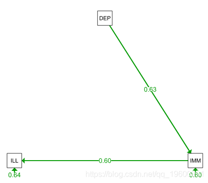
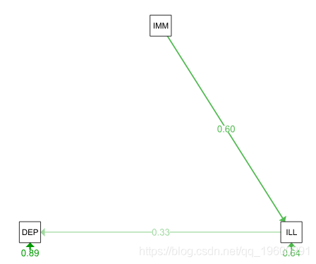
这两个简单的路径模型哪个更好？我们可以运行卡方检验。

## Chi Square Difference Test####         Df  AIC  BIC  Chisq Chisq diff Df diff Pr(>Chisq)## mod1fit  1 3786 3803   2.99## mod2fit  1 3981 3998 198.18        195       0     <2e-16 ***## ---## Signif. codes:  0 '***' 0.001 '**' 0.01 '*' 0.05 '.' 0.1 ' ' 1

可以看到模型2更好。让我们看一下模型2的一些属性。

# Goodness of fit measures##              fmin             chisq                df            pvalue##             0.198           198.180             1.000             0.000##    baseline.chisq       baseline.df   baseline.pvalue               cfi##           478.973             3.000             0.000             0.586##               tli              nnfi               rfi               nfi##            -0.243            -0.243             1.000             0.586##              pnfi               ifi               rni              logl##             0.195             0.587             0.586         -1986.510## unrestricted.logl              npar               aic               bic##         -1887.420             4.000          3981.020          3997.878##            ntotal              bic2             rmsea    rmsea.ci.lower##           500.000          3985.182             0.628             0.556##    rmsea.ci.upper      rmsea.pvalue               rmr        rmr_nomean##             0.703             0.000             0.176             0.176##              srmr       srmr_nomean             cn_05             cn_01##             0.176             0.176            10.692            17.740##               gfi              agfi              pgfi               mfi##             0.821            -0.075             0.137             0.821##              ecvi##             0.412

# Estimates of the model parameters##   lhs op rhs   est    se      z pvalue ci.lower ci.upper## 1 DEP  ~ ILL 0.330 0.042  7.817      0    0.247    0.413## 2 ILL  ~ IMM 0.600 0.036 16.771      0    0.530    0.670## 3 DEP ~~ DEP 0.889 0.056 15.811      0    0.779    1.000## 4 ILL ~~ ILL 0.639 0.040 15.811      0    0.560    0.718## 5 IMM ~~ IMM 0.998 0.000     NA     NA    0.998    0.998

# Modification indices##    lhs op rhs    mi    epc sepc.lv sepc.all sepc.nox## 1  DEP ~~ DEP   0.0  0.000   0.000    0.000    0.000## 2  DEP ~~ ILL 163.6 -0.719  -0.719   -0.720   -0.720## 3  DEP ~~ IMM 163.6  0.674   0.674    0.675    0.674## 4  ILL ~~ ILL   0.0  0.000   0.000    0.000    0.000## 5  ILL ~~ IMM    NA     NA      NA       NA       NA## 6  IMM ~~ IMM   0.0  0.000   0.000    0.000    0.000## 7  DEP  ~ ILL   0.0  0.000   0.000    0.000    0.000## 8  DEP  ~ IMM 163.6  0.675   0.675    0.675    0.676## 9  ILL  ~ DEP 163.6 -0.808  -0.808   -0.808   -0.808## 10 ILL  ~ IMM   0.0  0.000   0.000    0.000    0.000## 11 IMM  ~ DEP 143.8  0.666   0.666    0.666    0.666## 12 IMM  ~ ILL   0.0  0.000   0.000    0.000    0.000

非常感谢您阅读本文，有任何问题请在下面留言！