原文： http://tecdat.cn/?p=3897

文本分析：主题建模

library(tidyverse)theme_set( theme_bw())

目标

定义主题建模
解释Latent Dirichlet以及此过程的工作原理
演示如何使用LDA从一组已知主题中找到主题结构
演示如何使用LDA从一组未知主题中找到主题结构
确定k
选择适当参数的方法

主题建模

通常，当我们在线搜索信息时，有两种主要方法：

关键字 - 使用搜索引擎并输入与我们想要查找的内容相关的单词
链接。链接的页面可能共享相似或相关的内容。

另一种方法是通过主题搜索和探索文档。广泛的主题可能与文章中的各个部分（国家事务，体育）有关，但这些部分内或之间可能存在特定主题。

为此，我们需要有关每篇文章主题的详细信息。对该语料库进行手工编码将非常耗时，更不用说在开始编码之前需要知道文档的主题结构。

因此，我们可以使用概率主题模型，分析原始文本文档中的单词的统计算法来揭示语料库和单个文档本身的主题结构。在分析之前，它们不需要对文档进行任何手工编码或标记 - 相反，算法来自对文本的分析。

潜在Dirichlet分配

LDA假定语料库中的每个文档都包含在整个语料库中的混合主题。主题结构是隐藏的 - 我们只能观察文档和文字，而不是主题本身。因为结构是隐藏的（也称为潜在的），所以该方法试图在给定已知单词和文档的情况下推断主题结构。

食物和动物

假设您有以下句子：

我早餐吃了香蕉和菠菜。
我喜欢吃西兰花和香蕉。
龙猫和小猫很可爱。
我姐姐昨天收养了一只小猫。
看看这只可爱的仓鼠嚼着一块西兰花。

Latent Dirichlet分配是一种自动发现这些句子所包含的主题的方法。例如，给定这些句子并询问2个主题，LDA可能会产生类似的东西

句子1和2：100％主题A.
句子3和4：100％主题B.
句子5：60％主题A，40％主题B.
主题A：30％西兰花，15％香蕉，10％早餐，10％咀嚼，......
主题B：20％龙猫，20％小猫，20％可爱，15％仓鼠，......

您可以推断出主题A是关于食物的主题，主题B是关于可爱动物的主题。但是，LDA没有以这种方式明确地确定主题。它所能做的就是告诉你特定单词与主题相关的概率。

LDA文档结构

LDA将文档表示为以某些概率单词的主题组合。它假设文档以下列方式生成：在编写每个文档时，您

确定单词数N.
为文档选择主题（根据K个主题）
例如，假设我们上面有两个食物和可爱的动物主题。
通过以下方式生成文档中的每个单词：
首先选择一个主题（根据您在上面采样的分配;例如，您可以选择1/3概率的食物主题和2/3概率的可爱动物主题）。
然后使用主题生成单词本身（根据主题分配）。例如，食物主题可能输出概率为30％的“西兰花”，概率为15％的“香蕉”，依此类推。

我们怎么能在前面的例子中生成句子？生成文档D时：

D 将是一半关于食物和一半关于可爱动物。
选择5为D的单词数
从食物主题中选择第一个词，然后给出“西兰花”这个词。
选择第二个词来自可爱的动物主题，如“熊猫”。
选择第三个词来自可爱的动物主题，如“可爱”。
选择第四个词来源于食物主题，如“樱桃”。
从食物主题中选出第五个词，如“吃”。

因此，在LDA模型下生成的文件将是“可爱的熊猫吃樱桃和西兰花”（LDA使用的是词袋模型）。

通过LDA学习主题模型

现在假设您有一组文档。你选择了一些固定数量的K.

ķ是要发现的主题，我们希望使用LDA来学习每个文档的主题表示以及与每个主题相关联的单词。怎么做到这一点？一种方式（称为吉布斯采样）如下：

浏览每个文档，并将文档中的每个单词随机分配给K中的一个ķ 主题
但由于它是随机的，这不是一个非常准确的结构。
换句话说，在这一步中，我们假设除了当前单词之外的所有主题分配都是正确的，然后使用我们的文档生成模型更新当前单词的赋值。
重复上一步骤很多次，你最终会达到一个大致稳定的状态
您可以使用这些分配来估计两件事：

每个文档的主题（通过计算分配给该文档中每个主题的单词的比例）
与每个主题相关的单词（通过计算分配给每个主题的单词的比例）

具有已知主题结构的LDA

如果先验地知道一组文档的主题结构，LDA可能是有用的。

我们可以使用LDA和主题建模来发现章节与不同主题（即书籍）的关系。

作为预处理，我们将这些分为章节，使用tidytext unnest_tokens将它们分成单词，然后删除stop_words。我们将每一章都视为一个单独的“文档” 。

by_chapter <- books %>%group_by(title) %>%mutate(chapter = cumsum( str_detect(text, regex("^chapter ", ignore_case = TRUE)))) %>%ungroup() %>%count(title_chapter, word, sort = TRUE) %>%ungroup()## Joining, by = "word"word_counts## # A tibble: 104,721 × 3## title_chapter word n## <chr> <chr> <int>## 1 Great Expectations_57 joe 88## 2 Great Expectations_7 joe 70## 3 Great Expectations_17 biddy 63## 4 Great Expectations_27 joe 58## 5 Great Expectations_38 estella 58## 6 Great Expectations_2 joe 56## 7 Great Expectations_23 pocket 53## 8 Great Expectations_15 joe 50## 9 Great Expectations_18 joe 50## 10 The War of the Worlds_16 brother 50## # ... with 104,711 more rows

潜在狄利克雷分配(latnet Dirichlet allocation, LDA)模型

topicmodels包需要一个DocumentTermMatrix（来自tm包）。我们可以用cast_dtm函数转换为DocumentTermMatrix：

chapters_dtm## <<DocumentTermMatrix (documents: 193, terms: 18215)>>## Non-/sparse entries: 104721/3410774## Sparsity : 97%## Maximal term length: 19## Weighting : term frequency (tf)

现在我们准备创建一个四主题LDA模型。

chapters_lda <- LDA(chapters_dtm, k = 4, control = list(seed = 1234))chapters_lda## A LDA_VEM topic model with 4 topics.

在这种情况下，我们知道有四个主题，因为有四本书; 这是了解潜在主题结构的价值
seed = 1234设置随机迭代过程的起点。如果我们没有设置种子，那么每次运行脚本时我们都可以估算出略有不同的模型

我们从动词开始。

library(tidytext)chapters_lda_td <- tidy(chapters_lda)chapters_lda_td## # A tibble: 72,860 × 3## topic term beta## <int> <chr> <dbl>## 1 1 joe 5.830326e-17## 2 2 joe 3.194447e-57## 3 3 joe 4.162676e-24## 4 4 joe 1.445030e-02## 5 1 biddy 7.846976e-27## 6 2 biddy 4.672244e-69## 7 3 biddy 2.259711e-46## 8 4 biddy 4.767972e-03## 9 1 estella 3.827272e-06## 10 2 estella 5.316964e-65## # ... with 72,850 more rows

我们可以使用dplyr's top_n来查找每个主题中的前5个词：

top_n(5, beta) %>%ungroup() %>%arrange(topic, -beta)top_terms## # A tibble: 20 × 3## topic term beta## <int> <chr> <dbl>## 1 1 elizabeth 0.014107538## 2 1 darcy 0.008814258## 3 1 miss 0.008706741## 4 1 bennet 0.006947431## 5 1 jane 0.006497512

可视化

ggplot( aes(term, beta, fill = factor(topic))) +geom_bar(alpha = 0.8, stat

这些主题与四本书非常明显相关
“nemo”，“sea”和“nautilus”属于海底两万里
“jane”，“darcy”和“elizabeth”属于傲慢与偏见

另请注意，LDA()不会为每个主题分配任何标签。它们只是主题1,2,3和4. 我们可以推断这些与每本书有关，但它仅仅是我们的推论。

按文档分类

每一章都是本分析中的“文件”。因此，我们可能想知道哪些主题与每个文档相关联。我们可以把这些章节放回正确的书中吗？

chapters_lda_gamma## # A tibble: 772 × 3## document topic gamma## <chr> <int> <dbl>## 1 Great Expectations_57 1 1.351886e-05## 2 Great Expectations_7 1 1.470726e-05## 3 Great Expectations_17 1 2.117127e-05## 4 Great Expectations_27 1 1.919746e-05## 5 Great Expectations_38 1 3.544403e-01## 6 Great Expectations_2 1 1.723723e-05## 7 Great Expectations_23 1 5.507241e-01## 8 Great Expectations_15 1 1.682503e-02## 9 Great Expectations_18 1 1.272044e-05## 10 The War of the Worlds_16 1 1.084337e-05## # ... with 762 more rows

每行每个主题一个文档。现在我们已经有了这些文档分类，我们可以看到我们的无监督学习在区分四本书方面做得如何。

首先，我们将文档名称重新分为标题和章节：

chapters_lda_gamma <- chapters_lda_gamma %>%separate(document, c("title", "chapter"), sep = "_", convert = TRUE)chapters_lda_gamma## # A tibble: 772 × 4## title chapter topic gamma## * <chr> <int> <int> <dbl>## 1 Great Expectations 57 1 1.351886e-05## 2 Great Expectations 7 1 1.470726e-05## 3 Great Expectations 17 1 2.117127e-05## 4 Great Expectations 27 1 1.919746e-05## 5 Great Expectations 38 1 3.544403e-01## 6 Great Expectations 2 1 1.723723e-05## 7 Great Expectations 23 1 5.507241e-01## 8 Great Expectations 15 1 1.682503e-02## 9 Great Expectations 18 1 1.272044e-05## 10 The War of the Worlds 16 1 1.084337e-05## # ... with 762 more rows

然后我们检查每个章节的正确部分：

ggplot(chapters_lda_gamma, aes(gamma, fill = factor(topic))) +geom_histogram() +facet_wrap(~ title, nrow = 2)## `stat_bin()` using `bins = 30`. Pick better value with `binwidth`.

我们注意到，几乎所有来自“ 傲慢与偏见”，“世界大战 ”和“ 海底两万里 ”的章节都被确定为一个章节。

chapter_classifications <- chapters_lda_gamma %>%group_by(title, chapter) %>%top_n(1, gamma) %>%ungroup() %>%arrange(gamma)chapter_classifications## # A tibble: 193 × 4## title chapter topic gamma## <chr> <int> <int> <dbl>## 1 Great Expectations 54 3 0.4803234## 2 Great Expectations 22 4 0.5356506## 3 Great Expectations 31 4 0.5464851## 4 Great Expectations 23 1 0.5507241## 5 Great Expectations 33 4 0.5700737## 6 Great Expectations 47 4 0.5802089## 7 Great Expectations 56 4 0.5984806## 8 Great Expectations 38 4 0.6455341## 9 Great Expectations 11 4 0.6689600## 10 Great Expectations 44 4 0.6777974## # ... with 183 more rows

主题建模期望最大化算法中的一个重要步骤是将每个文档中的每个单词分配给一个主题。文档中的单词越多分配给该主题，通常，权重（gamma）将在该文档主题分类上。

具有未知主题结构的LDA

通常在使用LDA时，您实际上并不知道文档的基础主题结构。通常，这就是您首先使用LDA分析文本的原因。

美联社文章

数据是1992年发布的文章样本的文档术语矩阵。让我们将它们加载到R中并转换为整齐格式。

## 1 1 adding 1## 2 1 adult 2## 3 1 ago 1## 4 1 alcohol 1## 5 1 allegedly 1## 6 1 allen 1## 7 1 apparently 2## 8 1 appeared 1## 9 1 arrested 1## 10 1 assault 1## # ... with 302,021 more rows

为什么要先整理一下？因为原始的dtm包含停用词 - 我们想在建模数据之前删除它们。然后将数据转换回文档矩阵。

## Sparsity : 99%## Maximal term length: 18## Weighting : term frequency (tf)

每个主题的顶级词是什么样的？

group_by(topic) %>%top_n(5, beta) %>%ungroup() %>%arrange(topic, -beta)top_terms## # A tibble: 20 × 3## topic term beta## <int> <chr> <dbl>## 1 1 soviet 0.009502197## 2 1 government 0.009198486## 3 1 president 0.007046753## 4 1 united 0.006507324## 5 1 people 0.005402784## 6 2 people 0.007454587## 7 2 police 0.006433472## 8 2 city 0.003996852## 9 2 time 0.003369658## 10 2 school 0.003058213## 11 3 court 0.006850723## 12 3 bush 0.006510244## 13 3 president 0.005777216## 14 3 federal 0.005512805## 15 3 house 0.004657550## 16 4 percent 0.023766679## 17 4 million 0.012489935## 18 4 billion 0.009864418## 19 4 market 0.008402463## 20 4 prices 0.006693626top_terms %>%) +coord_flip()

这四个主题通常用于描述：

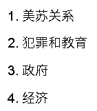
如果我们设置k=12

我们的结果如何变化？

group_by(topic) %>%top_n(5, beta) %>%ungroup() %>%arrange(topic, -beta)top_terms## # A tibble: 60 × 3## topic term beta## <int> <chr> <dbl>## 1 1 military 0.011691176## 2 1 united 0.011598436## 3 1 iraq 0.010618221## 4 1 president 0.009498227## 5 1 american 0.008253379## 6 2 dukakis 0.009819260## 7 2 bush 0.007300830## 8 2 campaign 0.006366915## 9 2 people 0.006098596## 10 2 school 0.005208529## # ... with 50 more rows

嗯，这些主题似乎更具体，但不易理解。

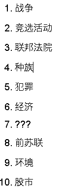
等。

LDA的某些方面是由直觉思维驱动的。但是我们可以提供辅助方法。

困惑度是概率模型预测样本的程度的统计量度。你估计LDA模型。然后给出由主题表示的理论单词分配，将其与实际主题或文档中单词的分配进行比较。

perplexity为给定模型计算该值的函数。

perplexity(ap_lda)## [1] 2301.814

但是，统计数据本身有点无意义。这种统计数据的好处在于比较不同模型的不同k的困惑度。具有最低困惑度的模型通常被认为是“最佳”。

让我们估算美联社数据集上的一系列LDA模型。

n_topics <- c(2, 4, 10, 20, 50, 100)ap_lda_compare <- n_topics %>%map(LDA, x = ap_dtm, control = list(seed = 1109))geom_point() +y = "Perplexity")

看起来100主题模型具有最低的困惑分数。这会产生什么样的主题？让我们看一下模型产生的前12个主题：

ap_lda_td <- tidy(ap_lda_compare[[6]])top_terms <- ap_lungroup() %>%arrange(topic, -beta)top_terms## # A tibble: 502 × 3## topic term beta## <int> <chr> <dbl>## 1 1 party 0.020029039## 2 1 communist 0.013810107## 3 1 government 0.013221069## 4 1 news 0.013036980## 5 1 soviet 0.011512086ggplot(aes(term, beta, fill = factor(topic))) +geom_bar(alpha = 0.8, stat = "identity", show.legend = FALSE) +facet_wrap(~ topic, scales = "free", ncol = 3) +coord_flip()