　　项目介绍

　　在这里我们主要对相关代码进行解释说明。我们将使用5个文件来实现 Faster-RCNN：

　　utils.py：关于检测框的绘制与计算;

　　demo.py：测试 utils.py 中的函数;

　　rpn.py：构造 RPN 网络;

　　train.py：训练 RPN 网络;

　　test.py：测试 RPN 网络。

　　utils.py 中的函数说明

　　1、wandhG

　　wandhG 中包含着 9 个预测框的宽度和长度(这是经过 kmeans 算法计算过的结果)。

　　import cv2

　　import numpy as np

　　import tensorflow as tf

　　wandhG = np.array([[ 74., 149.],

　　[ 34., 149.],

　　[ 86., 74.],

　　[109., 132.],

　　[172., 183.],

　　[103., 229.],

　　[149., 91.],

　　[ 51., 132.],

　　[ 57., 200.]], dtype=np.float32)

　　2、load_gt_boxes

　　def load_gt_boxes(path):

　　bbs = open(path).readlines()[1:]

　　roi = np.zeros([len(bbs), 4])

　　for iter_, bb in zip(range(len(bbs)), bbs):

　　bb = bb.replace('\n', '').split(' ')

　　bbtype = bb[0]

　　bba = np.array([float(bb[i]) for i in range(1, 5)])

　　ignore = int(bb[10])

　　ignore = ignore or (bbtype != 'person')

　　ignore = ignore or (bba[3] < 40)

　　bba[2] += bba[0]

　　bba[3] += bba[1]

　　roi[iter_, :4] = bba

　　return roi

　　load_gt_boxes() 函数返回一个 (-1, 4) 的数组，代表着多个检测物体的 ground truth boxes (即真实检测框)的左上角坐标和右下角坐标。

　　其中，我们需要输入一个路径，此路径下的 .txt 文件中包含着真实框的 (x, y, w, h)，x 表示真实框左上角的横坐标;y 表示真实框左上角的纵坐标;w 表示真实框的宽度;h 表示真实框的高度。

　　3、plot_boxes_on_image

　　def plot_boxes_on_image(show_image_with_boxes, boxes, color=[0, 0, 255], thickness=2):

　　for box in boxes:

　　cv2.rectangle(show_image_with_boxes,

　　pt1=(int(box[0]), int(box[1])),

　　pt2=(int(box[2]), int(box[3])), color=color, thickness=thickness)

　　show_image_with_boxes = cv2.cvtColor(show_image_with_boxes, cv2.COLOR_BGR2RGB)

　　return show_image_with_boxes

　　plot_boxes_on_image() 函数的输入有两个，分别是：需要被画上检测框的原始图片以及检测框的左上角和右下角的坐标。其输出为被画上检测框的图片。

　　4、compute_iou

　　def compute_iou(boxes1, boxes2):

　　left_up = np.maximum(boxes1[..., :2], boxes2[..., :2], )

　　right_down = np.minimum(boxes1[..., 2:], boxes2[..., 2:])

　　inter_wh = np.maximum(right_down - left_up, 0.0) # 交集的宽和长

　　inter_area = inter_wh[..., 0] * inter_wh[..., 1] # 交集的面积

　　boxes1_area = (boxes1[..., 2] - boxes1[..., 0]) * (boxes1[..., 3] - boxes1[..., 1]) # anchor 的面积

　　boxes2_area = (boxes2[..., 2] - boxes2[..., 0]) * (boxes2[..., 3] - boxes2[..., 1]) # ground truth boxes 的面积

　　union_area = boxes1_area + boxes2_area - inter_area # 并集的面积

　　ious = inter_area / union_area

　　return ious

　　compute_iou() 函数用来计算 IOU 值，即真实检测框与预测检测框(当然也可以是任意两个检测框)的交集面积比上它们的并集面积，这个值越大，代表这个预测框与真实框的位置越接近。用下面这个图片表示：

　　那么，left_up=[xmin2, ymin2];right_down=[xmax1, ymax1]。之后求出来这两个框的交集面积和并集面积，进而得到这两个框的 IOU 值。如果说得到的 IOU 值大于设置的正阈值，那么我们称这个预测框为正预测框(positive anchor)，其中包含着检测目标;如果说得到的 IOU 值小于于设置的负阈值，那么我们称这个预测框为负预测框(negative anchor)，其中包含着背景。

　　5、compute_regression

　　因为所有预测框的中心点位置(即特征图的每个块中心)以及尺寸(9个标准尺寸)都是固定的，那么这一定会导致获得的检测框很不准确。因此，我们希望创造一个映射，可以通过输入正预测框经过映射得到一个跟真实框更接近的回归框。

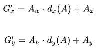
　　假设正预测框的坐标为 (Ax,Ay,Aw,Ah)(A_x, A_y, A_w, A_h)(Ax,Ay,Aw,Ah)，即正预测框左上角坐标为 (Ax,Ay)(A_x, A_y)(Ax,Ay)，宽度为 AwA_wAw，高度为 AhA_hAh;真实框的坐标为 (Gx,Gy,Gw,Gh)(G_x, G_y, G_w, G_h)(Gx,Gy,Gw,Gh);回归框的坐标为 (Gx′,Gy′,Gw′,Gh′)(G_x^{'}, G_y^{'}, G_w^{'}, G_h^{'})(Gx′,Gy′,Gw′,Gh′)。

　　那么，如何让正预测框变成回归框呢?

　　先做平移：

　　再做缩放：

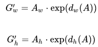
　　这里的 dx(A)d_x(A)dx(A)，dy(A)d_y(A)dy(A)，dw(A)d_w(A)dw(A) 和 dh(A)d_h(A)dh(A) 是我们需要学习的变换，称为回归变量。

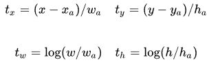
　　正预测框与真实框之间的平移量 (tx,ty)(t_x, t_y)(tx,ty) 与尺度因子 (tw,th)(t_w, t_h)(tw,th) 如下：

　　def compute_regression(box1, box2):

　　target_reg = np.zeros(shape=[4,])

　　w1 = box1[2] - box1[0]

　　h1 = box1[3] - box1[1]

　　w2 = box2[2] - box2[0]

　　h2 = box2[3] - box2[1]

　　target_reg[0] = (box1[0] - box2[0]) / w2

　　target_reg[1] = (box1[1] - box2[1]) / h2

　　target_reg[2] = np.log(w1 / w2)

　　target_reg[3] = np.log(h1 / h2)

　　return target_reg

　　6、decode_output

　　decode_output 函数的作用是，将一张图片上的 45*60*9 个预测框的平移量与尺度因子以及每个框的得分输入，得到每个正预测框对应的回归框(其实所有表示同一个检测目标的回归框都是近似重合的)。

　　def decode_output(pred_bboxes, pred_scores, score_thresh=0.5):

　　grid_x, grid_y = tf.range(60, dtype=tf.int32), tf.range(45, dtype=tf.int32)

　　grid_x, grid_y = tf.meshgrid(grid_x, grid_y)

　　grid_x, grid_y = tf.expand_dims(grid_x, -1), tf.expand_dims(grid_y, -1)

　　grid_xy = tf.stack([grid_x, grid_y], axis=-1)

　　center_xy = grid_xy * 16 + 8

　　center_xy = tf.cast(center_xy, tf.float32)

　　anchor_xymin = center_xy - 0.5 * wandhG

　　xy_min = pred_bboxes[..., 0:2] * wandhG[:, 0:2] + anchor_xymin

　　xy_max = tf.exp(pred_bboxes[..., 2:4]) * wandhG[:, 0:2] + xy_min

　　pred_bboxes = tf.concat([xy_min, xy_max], axis=-1)

　　pred_scores = pred_scores[..., 1]

　　score_mask = pred_scores > score_thresh

　　pred_bboxes = tf.reshape(pred_bboxes[score_mask], shape=[-1,4]).numpy()

　　pred_scores = tf.reshape(pred_scores[score_mask], shape=[-1,]).numpy()

　　return pred_scores, pred_bboxes

　　对于输入：

　　pred_bboxes：它的形状为 [1, 45, 60, 9, 4]，表示一共 45*60*9 个预测框，每个预测框都包含着两个平移量和两个尺度因子;

　　pred_scores：它的形状为 [1, 45, 60, 9, 2]，表示在 45*60*9 个预测框中，[1, i, j, k, 0] 表示第 i 行第 j 列中的第 k 个预测框中包含的是背景的概率;[1, i, j, k, 1] 表示第 i 行第 j 列中的第 k 个预测框中包含的是检测物体的概率。

　　其中，经过 meshgrid() 函数后，grid_x 的形状为 (45, 60)，grid_y 的性状也是 (45, 60)，它们的不同是：grid_x 由 45 行 range(60) 组成;grid_y 由 60 列 range(45) 组成。

　　经过 stack() 函数后，grid_xy 包含着所有特征图中小块的左上角的坐标，如 (0, 0)，(1, 0)，……，(59, 0)，(0, 1)，……，(59, 44)。

　　因为特征图中一个小块能表示原始图像中一块 16*16 的区域(也就是说，特征图中一个 1*1 的小块对应着原始图像上一个 16*16 的小块)，所以计算原始图像上每个小块的中心 center_xy 时，只需要用 grid_xy 乘 16 加 8 即可。

　　计算预测框的左上角坐标时，只需要用 center_xy 减去提前规定的预测框的宽度和长度(wandhG)的一半即可。

　　xy_min 和 xy_max 是回归框的左上角坐标和右下角坐标，它们的计算过程在 compute_regression() 函数那里已经讲过了，此处的 pred_bboxes 输入就是 compute_regression() 函数的输出，其中包含着每个框的平移量和尺度因子。然后将xy_min 和 xy_max 合并，得到新的 pred_bboxes，其中包含着回归框左上角坐标和右下角坐标。

　　pred_scores[…, 1] 指的是每个框中含有检测目标的概率(称为得分)，如果得分大于阈值，我们就认为这个框中检测到了目标，然后我们把这个框的坐标和得分提取出来，组成新的 pred_bboxes 和 pred_scores。

　　经过 decode_output 函数的输出为：

　　pred_score：其形状为 [-1, ]，表示每个检测框中的内容是检测物的概率。

　　pred_bboxes：其形状为 [-1, 4]，表示每个检测框的左上角和右下角的坐标。

　　7、nms

　　非极大值抑制(Non-Maximum Suppression，NMS)，顾名思义就是抑制不是极大值的元素，说白了就是去除掉那些重叠率较高但得分较低的预测框。

　　nms() 函数的作用是从选出的正预测框中进一步选出最好的 n 个预测框，其中，n 指图片中检测物的个数。其流程为：

　　取出所有预测框中得分最高的一个，并将这个预测框跟其他的预测框进行 IOU 计算;

　　将 IOU 值大于 0.1 的预测框视为与刚取出的得分最高的预测框表示了同一个检测物，故去掉;

　　重复以上操作，直到所有其他的预测框都被去掉为止。

　　def nms(pred_boxes, pred_score, iou_thresh):

　　"""

　　pred_boxes shape: [-1, 4]

　　pred_score shape: [-1,]

　　"""

　　selected_boxes = []

　　while len(pred_boxes) > 0:

　　max_idx = np.argmax(pred_score)

　　selected_box = pred_boxes[max_idx]

　　selected_boxes.append(selected_box)

　　pred_boxes = np.concatenate([pred_boxes[:max_idx], pred_boxes[max_idx+1:]])

　　pred_score = np.concatenate([pred_score[:max_idx], pred_score[max_idx+1:]])

　　ious = compute_iou(selected_box, pred_boxes)

　　iou_mask = ious <= 0.1

　　pred_boxes = pred_boxes[iou_mask]

　　pred_score = pred_score[iou_mask]

　　selected_boxes = np.array(selected_boxes)

　　return selected_boxes

　　demo.py

　　其实，到这儿，我们可以先用提供的人工标注的真实框坐标(左上角的坐标+宽+高)给图片中的检测目标画框来检验一下 utils.py 中的函数：

　　1、将 utils.py 中的函数导入

　　import cv2

　　import numpy as np

　　import tensorflow as tf

　　from PIL import Image

　　from utils import compute_iou, plot_boxes_on_image, wandhG, load_gt_boxes, compute_regression, decode_output

　　2、设置阈值与相关参数

　　pos_thresh = 0.5

　　neg_thresh = 0.1

　　iou_thresh = 0.5

　　grid_width = 16 # 网格的长宽都是16，因为从原始图片到 feature map 经历了16倍的缩放

　　grid_height = 16

　　image_height = 720

　　image_width = 960

　　3、读取图片与真实框坐标

　　image_path = "./synthetic_dataset/synthetic_dataset/image/2.jpg"

　　label_path = "./synthetic_dataset/synthetic_dataset/imageAno/2.txt"

　　gt_boxes = load_gt_boxes(label_path) # 把 ground truth boxes 的坐标读取出来

　　raw_image = cv2.imread(image_path) # 将图片读取出来 (高，宽，通道数)

　　我们可以尝试将真实框画在图片上：

　　image_with_gt_boxes = np.copy(raw_image) # 复制原始图片

　　plot_boxes_on_image(image_with_gt_boxes, gt_boxes) # 将 ground truth boxes 画在图片上

　　Image.fromarray(image_with_gt_boxes).show() # 展示画了 ground truth boxes 的图片

　　得到：

　　然后，我们需要再此复制原始图片用来求解每个预测框的得分和回归变量(平移量与尺度因子)。

　　4、每个预测框的得分和训练变量

　　## 因为得到的 feature map 的长宽都是原始图片的 1/16，所以这里 45=720/16，60=960/16。

　　target_scores = np.zeros(shape=[45, 60, 9, 2]) # 0: background, 1: foreground, ,

　　target_bboxes = np.zeros(shape=[45, 60, 9, 4]) # t_x, t_y, t_w, t_h

　　target_masks = np.zeros(shape=[45, 60, 9]) # negative_samples: -1, positive_samples: 1

　　################################### ENCODE INPUT #################################

　　## 将 feature map 分成 45*60 个小块

　　for i in range(45):

　　for j in range(60):

　　for k in range(9):

　　center_x = j * grid_width + grid_width * 0.5 # 计算此小块的中心点横坐标

　　center_y = i * grid_height + grid_height * 0.5 # 计算此小块的中心点纵坐标

　　xmin = center_x - wandhG[k][0] * 0.5 # wandhG 是预测框的宽度和长度，xmin 是预测框在图上的左上角的横坐标

　　ymin = center_y - wandhG[k][1] * 0.5 # ymin 是预测框在图上的左上角的纵坐标

　　xmax = center_x + wandhG[k][0] * 0.5 # xmax 是预测框在图上的右下角的纵坐标

　　ymax = center_y + wandhG[k][1] * 0.5 # ymax 是预测框在图上的右下角的纵坐标

　　# ignore cross-boundary anchors

　　if (xmin > -5) & (ymin > -5) & (xmax < (image_width+5)) & (ymax < (image_height+5)):

　　anchor_boxes = np.array([xmin, ymin, xmax, ymax])

　　anchor_boxes = np.expand_dims(anchor_boxes, axis=0)

　　# compute iou between this anchor and all ground-truth boxes in image.

　　ious = compute_iou(anchor_boxes, gt_boxes)

　　positive_masks = ious > pos_thresh

　　negative_masks = ious < neg_thresh

　　if np.any(positive_masks):

　　plot_boxes_on_image(encoded_image, anchor_boxes, thickness=1)

　　print("=> Encoding positive sample: %d, %d, %d" %(i, j, k))

　　cv2.circle(encoded_image, center=(int(0.5*(xmin+xmax)), int(0.5*(ymin+ymax))),

　　radius=1, color=[255,0,0], thickness=4) # 正预测框的中心点用红圆表示

　　target_scores[i, j, k, 1] = 1. # 表示检测到物体

　　target_masks[i, j, k] = 1 # labeled as a positive sample

　　# find out which ground-truth box matches this anchor

　　max_iou_idx = np.argmax(ious)

　　selected_gt_boxes = gt_boxes[max_iou_idx]

　　target_bboxes[i, j, k] = compute_regression(selected_gt_boxes, anchor_boxes[0])

　　if np.all(negative_masks):

　　target_scores[i, j, k, 0] = 1. # 表示是背景

　　target_masks[i, j, k] = -1 # labeled as a negative sample

　　cv2.circle(encoded_image, center=(int(0.5*(xmin+xmax)), int(0.5*(ymin+ymax))),

　　radius=1, color=[0,0,0], thickness=4) # 负预测框的中心点用黑圆表示

　　Image.fromarray(encoded_image).show()

　　在这里，我们只考虑部分位置符合条件的预测框，如果这个预测框和某一个真实框(一张图片中可以有多个真实框，这取决于图片中检测目标的个数)的 IOU 值大于给定的正阈值，我们就称这个预测框为这个真实框的正预测框;如果这个预测框和某一个真实框的 IOU 值小于给定的负阈值，我们就称这个预测框为这个真实框的负预测框。

　　如果一个预测框为某真实框的正预测框，我们就将它的检测目标得分赋1，将其标记为正样本，并计算这个正预测框和它所对应的真实框之间的回归变量;如果一个预测框对所有真实框来说都是负预测框，我们就将它的背景得分赋-1，并将其标记为负样本。

　　最终得到：

　　5、根据每个预测框的得分和训练变量得到回归框

　　############################## FASTER DECODE OUTPUT ###############################

　　faster_decode_image = np.copy(raw_image)

　　pred_bboxes = np.expand_dims(target_bboxes, 0).astype(np.float32)

　　pred_scores = np.expand_dims(target_scores, 0).astype(np.float32)

　　pred_scores, pred_bboxes = decode_output(pred_bboxes, pred_scores)

　　plot_boxes_on_image(faster_decode_image, pred_bboxes, color=[255, 0, 0]) # red boundig box

　　Image.fromarray(np.uint8(faster_decode_image)).show()

　　得到：

　　可见，回归框和真实框的位置差不多。

　　rpn.py

　　rpn.py 文件是用来建立 RPN 网络的，在这里，我们对原始的 RPN 网络进行了一些改进，其代码如下：

　　import tensorflow as tf

　　class RPNplus(tf.keras.Model):

　　# VGG_MEAN = [103.939, 116.779, 123.68]

　　def __init__(self):

　　super(RPNplus, self).__init__()

　　# conv1

　　self.conv1_1 = tf.keras.layers.Conv2D(64, 3, activation='relu', padding='same')

　　self.conv1_2 = tf.keras.layers.Conv2D(64, 3, activation='relu', padding='same')

　　self.pool1 = tf.keras.layers.MaxPooling2D(2, strides=2, padding='same')

　　# conv2

　　self.conv2_1 = tf.keras.layers.Conv2D(128, 3, activation='relu', padding='same')

　　self.conv2_2 = tf.keras.layers.Conv2D(128, 3, activation='relu', padding='same')

　　self.pool2 = tf.keras.layers.MaxPooling2D(2, strides=2, padding='same')

　　# conv3

　　self.conv3_1 = tf.keras.layers.Conv2D(256, 3, activation='relu', padding='same')

　　self.conv3_2 = tf.keras.layers.Conv2D(256, 3, activation='relu', padding='same')

　　self.conv3_3 = tf.keras.layers.Conv2D(256, 3, activation='relu', padding='same')

　　self.pool3 = tf.keras.layers.MaxPooling2D(2, strides=2, padding='same')

　　# conv4

　　self.conv4_1 = tf.keras.layers.Conv2D(512, 3, activation='relu', padding='same')

　　self.conv4_2 = tf.keras.layers.Conv2D(512, 3, activation='relu', padding='same')

　　self.conv4_3 = tf.keras.layers.Conv2D(512, 3, activation='relu', padding='same')

　　self.pool4 = tf.keras.layers.MaxPooling2D(2, strides=2, padding='same')

　　# conv5

　　self.conv5_1 = tf.keras.layers.Conv2D(512, 3, activation='relu', padding='same')

　　self.conv5_2 = tf.keras.layers.Conv2D(512, 3, activation='relu', padding='same')

　　self.conv5_3 = tf.keras.layers.Conv2D(512, 3, activation='relu', padding='same')

　　self.pool5 = tf.keras.layers.MaxPooling2D(2, strides=2, padding='same')

　　## region_proposal_conv

　　self.region_proposal_conv1 = tf.keras.layers.Conv2D(256, kernel_size=[5,2],

　　activation=tf.nn.relu,