使用Word2vec和Keras在Twitter上进行情感分析
1 简介
word2vec是由Google开发的一组深度学习模型,目的是捕获单词的上下文,同时提出一种非常有效的预处理原始文本数据的方法。该模型将大量文档(例如推文或新闻文章)作为输入,并生成通常具有数百个维度的向量空间。在向量空间中,为语料库中的每个单词分配了唯一的向量。
word2vec背后的强大概念是向量空间中彼此接近的词向量代表的词不仅具有相同的含义,而且具有相同的上下文。
我发现单词向量表示的有趣之处在于它自动嵌入了我们通常必须手工制作的一些功能。由于word2vec依赖于深度神经网络来检测模式,因此我们可以依靠它来检测不同抽象级别上的多个功能。
下面两张图表中,在降维后投影在2D空间上的某些单词向量可视化
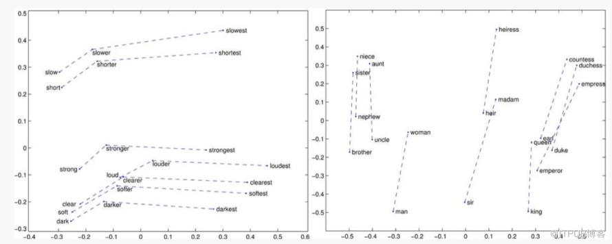
在右图上,具有相似含义,概念和上下文的词被组合在一起。例如,侄女,阿姨和姐姐彼此接近,因为它们描述了女性和家庭关系。同样,将伯爵夫人,公爵夫人和皇后归为一类,因为它们代表女性皇室。从该图表可以看到的第二件事是单词之间的几何距离转换了语义关系。例如,向量女人-男人与向量女王/王后在某种程度上是共线的,这意味着word2vec能够推断单词之间的不同关系。
左图与右图非常相似,不同之处在于它可以翻译单词之间的语法关系。慢-最慢 = 短-最短就是这样的例子。
在更一般的层面上,word2vec在单词之间嵌入了非平凡的语义和语法关系。这导致保留了丰富的上下文。
在本文中,将利用word2vec的功能来构建情感分类器。将使用150万条推文的大型数据集,其中每条推文在标记为正时标记为1,在标记为负时标记为0。word2vec模型将学习该语料库中每个单词的表示,也将用于将推文(即句子)转换为向量的表示。然后,我们将使用这种新的推文表示法来训练Keras的神经网络分类器。
2 环境设置和数据准备
在 Ubuntu 16.04 LTS计算机上创建了一个名为nlp的conda虚拟环境。python版本是2.7。
conda create -n nlp python=2.7 anaconda
激活环境
source activate nlp
在此虚拟环境中,我们需要安装以下库:
pip install --upgrade gensim
pip install nltk
pip install tqdm
pip install --upgrade https://storage.googleapis.com/tensorflow/linux/cpu/tensorflow-1.0.1-cp27-none-linux_x86_64.whl
pip install keras
pip install bokeh
其中
gensim是一种自然语言处理python库。它使文本挖掘,清理和建模变得非常容易。此外,它提供了word2vec模型的实现。
Keras是用Python编写的高级神经网络API,能够在TensorFlow或Theano上运行。我们将使用它来训练我们的情绪分类器。在本教程中,它将在TensorFlow上运行。
TensorFlow是一个用于机器学习的开源软件库。它是由Google开发的,旨在满足他们对能够构建和训练神经网络的系统的需求。
Bokeh是一个Python交互式可视化库,以现代Web浏览器为对象进行演示。其目标是以D3.js的样式提供优雅,简洁的新颖图形构造,并通过在大型或流数据集上的高性能交互性来扩展此功能。
-
tqdm是很酷的进度条实用程序包,用来监视数据帧的创建。
可以之后,可以从这里下载数据集。这是一个包含160万行的csv文件。每行除其他外还具有推文的文本和相应的情感。
让我们加载python库并查看数据集。
import pandas as pd # provide sql-like data manipulation tools. very handy.
pd.options.mode.chained_assignment = None
import numpy as np # high dimensional vector computing library.
from copy import deepcopy
from string import punctuation
from random import shuffle

import gensim
from gensim.models.word2vec import Word2Vec # the word2vec model gensim class
LabeledSentence = gensim.models.doc2vec.LabeledSentence # we'll talk about this down below

from tqdm import tqdm
tqdm.pandas(desc="progress-bar")

from nltk.tokenize import TweetTokenizer # a tweet tokenizer from nltk.
tokenizer = TweetTokenizer()

from sklearn.model_selection import train_test_split
from sklearn.feature_extraction.text import TfidfVectorizer
加载并提取文本需要两列内容:
情感:0 / 1变量
tweet的文本:字符型
def ingest():
    data = pd.read_csv('./tweets.csv')
    data.drop(['ItemID', 'SentimentSource'], axis=1, inplace=True)
    data = data[data.Sentiment.isnull() == False]
    data['Sentiment'] = data['Sentiment'].map(int)
    data = data[data['SentimentText'].isnull() == False]
    data.reset_index(inplace=True)
    data.drop('index', axis=1, inplace=True)
    print 'dataset loaded with shape', data.shape
    return data

data = ingest()
data.head(5)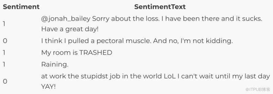
SentimenText的格式是无用的,需要被标记和清理。我们将限制在100万条。下面标记化函数,它将每条tweet拆分为标记,并删除用户@、#和url。这些元素在tweet中非常常见,但遗憾的是,它们没有为任务提供足够的语义信息,因此对这些文本字符串进行删除。
def tokenize(tweet):
    try:
        tweet = unicode(tweet.decode('utf-8').lower())
        tokens = tokenizer.tokenize(tweet)
        tokens = filter(lambda t: not t.startswith('@'), tokens)
        tokens = filter(lambda t: not t.startswith('#'), tokens)
        tokens = filter(lambda t: not t.startswith('http'), tokens)
        return tokens
    except:
        return 'NC'
现在应该清理标记化的结果,以删除带有“NC”的行,这是由标记化错误导致的。
def postprocess(data, n=1000000):
    data = data.head(n)
    data['tokens'] = data['SentimentText'].progress_map(tokenize)  ## progress_map is a variant of the map function plus a progress bar. Handy to monitor DataFrame creations.
    data = data[data.tokens != 'NC']
    data.reset_index(inplace=True)
    data.drop('index', inplace=True, axis=1)
    return data

data = postprocess(data)
3 建立word2vec模型
首先,我们定一个训练集和测试集
x_train, x_test, y_train, y_test = train_test_split(np.array(data.head(n).tokens),
                                                    np.array(data.head(n).Sentiment), test_size=0.2)
在将tokens列表输入到word2vec模型之前,我们必须先将它们转换为带标签的句子对象
def labelizeTweets(tweets, label_type):
    labelized = []
    for i,v in tqdm(enumerate(tweets)):
        label = '%s_%s'%(label_type,i)
        labelized.append(LabeledSentence(v, [label]))
    return labelized

x_train = labelizeTweets(x_train, 'TRAIN')
x_test = labelizeTweets(x_test, 'TEST')
x_train中的第一个元素
x_train[0]

# TaggedDocument(words=[u'thank', u'you', u'!', u'im', u'just', u'a', u'tad', u'sad', u'u', u'r', u'off', u'the', u'market', u'tho', u'...'], tags=['TRAIN_0'])
所以每个元素基本上都是一些具有两个属性的对象:一个列表(tokens)和一个标签。现在我们准备从x_train即语料库构建word2vec模型。
tweet_w2v = Word2Vec(size=n_dim, min_count=10)
tweet_w2v.build_vocab([x.words for x in tqdm(x_train)])
tweet_w2v.train([x.words for x in tqdm(x_train)])
在第一行中,用向量空间的维数初始化模型(我们将其设置为200),
在第二行中创建词汇表。
在第三行,模型被训练,即它的权重被更新。在tweet的语料库上建立模型并进行训练后,我们就可以使用它将单词转换为向量。这里有一个例子
tweet_w2v['good']

#  array([-1.04697919,  0.79274398,  0.23612066,  0.05131698,  0.0884205 ,
#        -0.08569263,  1.45526719,  0.42579028, -0.34688851, -0.08249081,
#         0.45873582,  2.36241221,  1.05570769, -1.99480379, -1.80352235,
#        -0.15522274, -0.20937157, ..., 1.58423829], dtype=float32)
ps:我们只能得到语料库中单词的向量。我们之前谈到过语义关系。Word2Vec gensim实现提供了一个很酷的方法most_similar。给定一个单词,这个方法返回前n个相似的单词。这是一个有趣的特性。让我们在一些单词上试一下
tweet_w2v.most_similar('good')

# [(u'goood', 0.7355118989944458),
#  (u'great', 0.7164269685745239),
#  (u'rough', 0.656904935836792),
#  (u'gd', 0.6395257711410522),
#  (u'goooood', 0.6351571083068848),
#  (u'tough', 0.6336284875869751),
#  (u'fantastic', 0.6223267316818237),
#  (u'terrible', 0.6179217100143433),
#  (u'gooood', 0.6099461317062378),
#  (u'gud', 0.6096700429916382)]

tweet_w2v.most_similar('bar')

# [(u'pub', 0.7254607677459717),
#  (u'restaurant', 0.7147054076194763),
#  (u'cafe', 0.7105239629745483),
#  (u'table', 0.6781781911849976),
#  (u'ranch', 0.6559066772460938),
#  (u'club', 0.6470779180526733),
#  (u'panera', 0.6464691162109375),
#  (u'bakery', 0.6429882049560547),
#  (u'grill', 0.6425997018814087),
#  (u'gate', 0.6346235275268555)]

tweet_w2v.most_similar('facebook')

# [(u'fb', 0.8862842321395874),
#  (u'myspace', 0.8414138555526733),
#  (u'bebo', 0.7763116359710693),
#  (u'yahoo', 0.7672140598297119),
#  (u'msn', 0.7638905048370361),
#  (u'twitter', 0.7276350259780884),
#  (u'tumblr', 0.7209618091583252),
#  (u'flickr', 0.712773323059082),
#  (u'skype', 0.7116719484329224),
#  (u'aim', 0.7065393924713135)]

tweet_w2v.most_similar('iphone')

# [(u'itouch', 0.7907721996307373),
#  (u'blackberry', 0.7342787981033325),
#  (u'firmware', 0.7048080563545227),
#  (u'jailbreak', 0.7042940855026245),
#  (u'mac', 0.7014051675796509),
#  (u'3gs', 0.697465717792511),
#  (u'pc', 0.6917887330055237),
#  (u'upgrade', 0.6857078075408936),
#  (u'mms', 0.6838993430137634),
#  (u'3.0', 0.6824861764907837)]
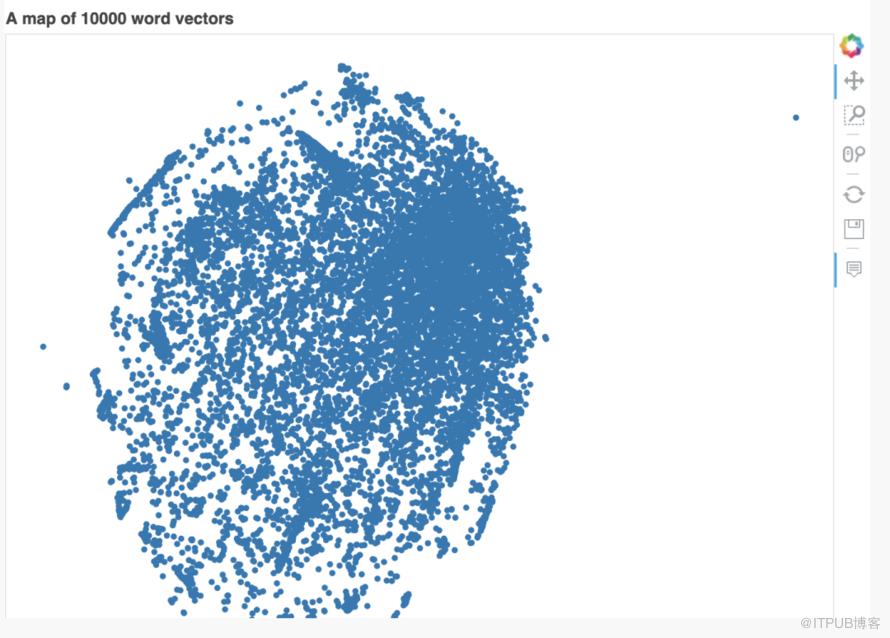
那么如何将这些词向量形象化呢? 我们首先要用t-SNE把它们的维数减小到2。然后,我们使用一个交互式的可视化工具,如Bokeh,我们可以直接映射到二维平面上,并与他们进行交互:
importing bokeh library for interactive dataviz
import bokeh.plotting as bp
from bokeh.models import HoverTool, BoxSelectTool
from bokeh.plotting import figure, show, output_notebook

# defining the chart
output_notebook()
plot_tfidf = bp.figure(plot_width=700, plot_height=600, title="A map of 10000 word vectors",
    tools="pan,wheel_zoom,box_zoom,reset,hover,previewsave",
    x_axis_type=None, y_axis_type=None, min_border=1)

# getting a list of word vectors. limit to 10000. each is of 200 dimensions
word_vectors = [tweet_w2v[w] for w in tweet_w2v.wv.vocab.keys()[:5000]]

# dimensionality reduction. converting the vectors to 2d vectors
from sklearn.manifold import TSNE
tsne_model = TSNE(n_components=2, verbose=1, random_state=0)
tsne_w2v = tsne_model.fit_transform(word_vectors)

# putting everything in a dataframe
tsne_df = pd.DataFrame(tsne_w2v, columns=['x', 'y'])
tsne_df['words'] = tweet_w2v.wv.vocab.keys()[:5000]

# plotting. the corresponding word appears when you hover on the data point.
plot_tfidf.scatter(x='x', y='y', source=tsne_df)
hover = plot_tfidf.select(dict(type=HoverTool))
hover.tooltips={"word": "@words"}
show(plot_tfidf)
4 建立一个情感分类器
为了对推文进行分类,我们还必须将其转换为向量,由于我们知道组成推文的每个单词的向量表示形式,因此我们必须将这些向量“组合”在一起,并获得一个代表整个推文的新向量。
第一种方法是将单词向量平均在一起。但是有一个更好的解决方案是计算一个加权平均值,其中每个权重都给出了单词相对于语料库的重要性,这样的权重可以使tf-idf得分。下面构建一个TF-IDF矩阵。
print 'building tf-idf matrix ...'
vectorizer = TfidfVectorizer(analyzer=lambda x: x, min_df=10)
matrix = vectorizer.fit_transform([x.words for x in x_train])
tfidf = dict(zip(vectorizer.get_feature_names(), vectorizer.idf_))
print 'vocab size :', len(tfidf)
def buildWordVector(tokens, size):
    vec = np.zeros(size).reshape((1, size))
    count = 0.
    for word in tokens:
        try:
            vec += tweet_w2v[word].reshape((1, size)) * tfidf[word]
            count += 1.
        except KeyError: # handling the case where the token is not
                         # in the corpus. useful for testing.
            continue
    if count != 0:
        vec /= count
    return vec
from sklearn.preprocessing import scale
train_vecs_w2v = np.concatenate([buildWordVector(z, n_dim) for z in tqdm(map(lambda x: x.words, x_train))])
train_vecs_w2v = scale(train_vecs_w2v)

test_vecs_w2v = np.concatenate([buildWordVector(z, n_dim) for z in tqdm(map(lambda x: x.words, x_test))])
test_vecs_w2v = scale(test_vecs_w2v)
现在我们应该准备将这些向量输入到神经网络分类器中。实际上,使用Keras定义层和激活功能非常容易。这是一个基本的2层体系结构。
model = Sequential()
model.add(Dense(32, activation='relu', input_dim=200))
model.add(Dense(1, activation='sigmoid'))
model.compile(optimizer='rmsprop',
              loss='binary_crossentropy',
              metrics=['accuracy'])

model.fit(train_vecs_w2v, y_train, epochs=9, batch_size=32, verbose=2)
现在已经对模型进行了训练,让我们在测试集中对其进行评估:
score = model.evaluate(test_vecs_w2v, y_test, batch_size=128, verbose=2)
print(score[1])
# 0.78984528240986307
5 结论
-
在这篇文章中,我们探索了执行情感分析的不同工具:我们使用word2vec和Keras构建了一个tweet情感分类器。
-
这两种工具的结合使分类模型的准确性达到了79%。
-
该Keras模型可以保存并用于其他tweet数据,例如通过tweepy API提取的流数据。将该模型也包装在带有一些D3.js可视化仪表板的Web应用程序周围可能会很有趣。
关于此分类器的改进,我们可以研究doc2vec模型,该模型从句子和段落中提取向量。
参考文献
https://www.ahmedbesbes.com/blog/sentiment-analysis-with-keras-and-word-2-vec
https://drive.google.com/uc?id=0B04GJPshIjmPRnZManQwWEdTZjg&export=download



原文作者:ChallengeHub;如有侵权,请联系管理员删除。

