Pytorch框架下的Transforemr时间序列预测实例

前言
作者介绍:Answer,大四,187cm,目前就读于郑州大学,保研至中国人民大学,专业为流行病与卫生统计,爱好打篮球,撸代码。

作者本人照片
前段时间作者使用Transformer模型做了一下时间序列预测,在此分享一下。本文主要内容为代码,Transformer理论部分请参考原文献及其他文章。
1.项目背景
如今文献数据库收录的科学文献的数量飞速增长,科研工作者评估论文科学影响力的最直接、最常用的度量标准是文献被引量,本文希望基于Transformer模型预测科学文献的文献被引量,进而衡量科技论文的潜在影响力。

本文使用的文献数据采集于Web of Science网站,表1和图1展示了文献数据特征,其中包括每一条文献1970年至2019年的被引量序列,以及一些时间序列特征之外的文献特征。

2.Transformer 模型简介
Transformer模型最初由Google团队于2017年提出并应于机器翻译[1],其抛弃了传统循环神经网络提取序列信息的方式,开创性的提出了注意力机制实现快速并行,改进了循环神经网络训练慢的缺点。
本文建模时仅使用了Transformer的Encoder部分,最后连接一个全连接层将张量投影为 [batch_size, output_len] 的形式。 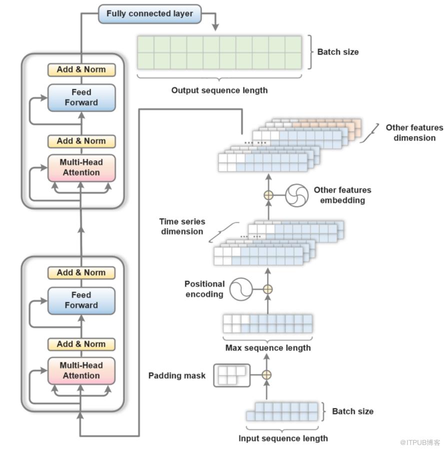
3.数据预处理
以下是本次建模用到的库~
 #### 调用库 ####
 import pandas as pd
 import torch
 import torch.nn as nn
 import numpy as np
 import time
 import math
 from matplotlib import pyplot
 from sklearn.model_selection import train_test_split
 import os
 os.environ["KMP_DUPLICATE_LIB_OK"] = "TRUE"
 torch.manual_seed(0)
 np.random.seed(0)
Transformer模型应用于自然语言处理领域时,其输入数据通常为不同长度的句子。对此,原作者在文献“Attention is all you need”中提出了掩码填充(Padding mask)机制,其原理是将一个负无穷大的数字填充到这些位置,将句子补为等长数据,通过多头注意力机制中的softmax函数将填充位置的权值变成0,使模型能够有效处理不等长数据。本文使用的文献数据中每篇文献1970到2019年的被引量序列与文本数据类似,由于不同文献的发表年份不同,被引序列的长度也不一致,所以本文将1970到出版年份之间的部分进行了掩码填充。
 #### 获取需要掩码的位置 ####
 def get_padding_mask(input):  #因为出版之前不存在被引用的可能,所以需要将论文出版年之前的位置掩码
     input1 = pd.DataFrame(input)
     for pub in range(1970, 2020):
         if pub == 1970:
             input1.loc[input1['出版年'] == 1970, '1970':'2019'] = 0
         else:
             input1.loc[input1['出版年'] == 1970, '1970':str(pub - 1)] = 1  # 1 转换为 bool 是 TRUE,表示掩码
             input1.loc[input1['出版年'] == 1970, str(pub):'2019'] = 0
     input1 = input1.loc[:, '1970':'2019']
     return input1
相比于传统的循环神经网络和卷积神经网络,Transformer模型提出了全新的位置编码(Positional encoding)机制来捕获输入数据间的时间序列信息。其原理是将不同频率的正弦和余弦函数作为“位置编码”添加到归一化之后的输入序列中,使得Transformer模型中的多头注意力机制能够充分捕获维度更为丰富的时间序列信息。位置编码的维数是可以优化的超参数。
 #### positional encoding ####
 class PositionalEncoding(nn.Module):
     def __init__(self, d_model, max_len=50):
         super(PositionalEncoding, self).__init__()
         pe = torch.zeros(max_len, d_model)
         position = torch.arange(0, max_len, dtype=torch.float).unsqueeze(1)
         div_term = torch.exp(torch.arange(0, d_model, 2).float() * (-math.log(10000.0) / d_model))
         pe[:, 0::2] = torch.sin(position * div_term)
         pe[:, 1::2] = torch.cos(position * div_term)
         pe = pe.unsqueeze(0).transpose(0, 1)
         # pe.requires_grad = False
         self.register_buffer('pe', pe)

     def forward(self, x):
         return x + self.pe[:x.size(0), :]
由于一篇科学文献除时间序列特征外,还具有作者影响力、出版期刊、出版年份等多样的特征,而这些特征对文献被引量的预测又具有极其重要的作用。故此本文将文献特征中的定性特征转换为0-1变量,定量变量保持不变,并将这些特征与时间序列特征合并起来,一同输入到Transformer模型当中。(这一部分的代码作者还没来得及写)
以下代码用于读取原数据并划分训练、测试数据。
 #### 生成训练、测试数据 ####
 def get_data():
     data = pd.read_csv('cleaned_data.csv', encoding='GBK', chunksize=1000)  # 数据量有点大,所以分批读入
     data = pd.concat(data, ignore_index=True)
     data = data.dropna()  # 删除缺失数据
     for i in range(1971, 2020):  # 由每一年的数值变成累积数值
         data[str(i)] = data[str(i - 1)] + data[str(i)]
     data = data[data['出版年'] <= 2010]
     data = data[data['2015'] > 0]
     data.reset_index(inplace=True, drop=True)
     data = data.loc[0:3001, :]  # 这里可以选用数据量
     train_data, test_data = train_test_split(data, train_size=0.8, random_state=10)
     data.reset_index(inplace=True, drop=True)
     train_data.reset_index(inplace=True, drop=True)
     test_data.reset_index(inplace=True, drop=True)
     train_data1 = train_data  # 这里复制了一份数据,方便后续获取需要掩码的位置
     test_data1 = test_data
     train_data = train_data.loc[:, '1970':'2019']
     test_data = test_data.loc[:, '1970':'2019']
     max1 = max(max(test_data.max()), max(train_data.max()))  # 用于归一化处理
     train_data = train_data / max1
     test_data = test_data / max1

     train_padding = get_padding_mask(train_data1)  # 调用 get_padding_mask 函数
     test_padding = get_padding_mask(test_data1)
     train_seq = torch.from_numpy(np.array(train_data.iloc[:, :-output_window]))
     train_label = torch.from_numpy(np.array(train_data.iloc[:, output_window:]))

     test_seq = torch.from_numpy(np.array(test_data.iloc[:, :-output_window]))
     test_label = torch.from_numpy(np.array(test_data.iloc[:, output_window:]))

     train_padding = torch.from_numpy(np.array(train_padding.iloc[:, :-output_window]))
     test_padding = torch.from_numpy(np.array(test_padding.iloc[:, :-output_window]))

     train_sequence = torch.stack((train_seq, train_label, train_padding), dim=1).type(torch.FloatTensor)
     test_data = torch.stack((test_seq, test_label, test_padding), dim=1).type(torch.FloatTensor)
     return train_sequence.to(device), test_data.to(device), max1
4.Transformer模型主体部分
 #### model stracture ####
 class TransAm(nn.Module):
     def __init__(self, feature_size=512, num_layers=1, dropout=0):  # feature_size 表示特征维度(必须是head的整数倍), num_layers 表示 Encoder_layer 的层数, dropout 用于防止过你和
         super(TransAm, self).__init__()
         self.model_type = 'Transformer'
         self.src_mask = None
         self.pos_encoder = PositionalEncoding(feature_size)  #位置编码前要做归一化,否则捕获不到位置信息
         self.encoder_layer = nn.TransformerEncoderLayer(d_model=feature_size, nhead=8, dropout=dropout)  # 这里用了八个头
         self.transformer_encoder = nn.TransformerEncoder(self.encoder_layer, num_layers=num_layers)
         self.decoder = nn.Linear(feature_size, 1)  # 这里用全连接层代替了decoder, 其实也可以加一下Transformer的decoder试一下效果
         self.init_weights()
         self.src_key_padding_mask = None  # 后面用了掩码~

     def init_weights(self):
         initrange = 0.1
         self.decoder.bias.data.zero_()
         self.decoder.weight.data.uniform_(-initrange, initrange)

     def forward(self, src, src_padding):
         if self.src_key_padding_mask is None:
             mask_key = src_padding.bool()
             self.src_key_padding_mask = mask_key

         src = self.pos_encoder(src)
         output = self.transformer_encoder(src, self.src_mask, self.src_key_padding_mask)
         output = self.decoder(output)
         return output
5.训练测试
5.1 定义训练部分
 #### 定义训练函数 ####
 def train(train_data):
     model.train()  # Turn on the train mode
     total_loss = 0.
     start_time = time.time()

     for batch, i in enumerate(range(0, len(train_data) - 1, batch_size)):
         data, targets, key_padding_mask = get_batch(train_data, i, batch_size)
         optimizer.zero_grad()
         output = model(data, key_padding_mask)

         if calculate_loss_over_all_values:
             loss = criterion(output, targets)
         else:  # Pytorch这里面的输入和输出序列要求是等长的,否则会报错,这一部分适用于计算输出序列中预测部分的 loss
             loss = criterion(output[-output_window:], targets[-output_window:])

         loss.backward()
         torch.nn.utils.clip_grad_norm_(model.parameters(), 0.5)
         optimizer.step()

         total_loss += loss.item()
         log_interval = int(len(train_data) / batch_size / 5)
         if batch % log_interval == 0 and batch > 0:
             cur_loss = total_loss / log_interval
             elapsed = time.time() - start_time
             print('| epoch {:3d} | {:5d}/{:5d} batches | '
                   'lr {:02.6f} | {:5.2f} ms | '
                   'loss {:5.5f}'.format(
                 epoch, batch, len(train_data) // batch_size, scheduler.get_lr()[0],
                               elapsed * 1000 / log_interval,
                 cur_loss))  # , math.exp(cur_loss)
             total_loss = 0
             start_time = time.time()
5.2 定义测试部分
 #### 定义测试函数 ####
 def evaluate(eval_model, data_source):
     eval_model.eval()  # Turn on the evaluation mode
     total_loss = 0.
     eval_batch_size = 50
     with torch.no_grad():
         for i in range(0, len(data_source) - 1, eval_batch_size):
             data, targets, key_padding_mask = get_batch(data_source, i, eval_batch_size)
             output = eval_model(data, key_padding_mask)
             if calculate_loss_over_all_values:
                 total_loss += len(data[0]) * criterion(output, targets).cpu().item()
             else:
                 total_loss += len(data[0]) * criterion(output[-output_window:], targets[-output_window:]).cpu().item()
     return total_loss / len(data_source)
5.3 训练过程可视化
 #### 训练过程可视化 ####
 def plot_and_loss(eval_model, data_source, epoch):
     eval_model.eval()
     total_loss = 0.
     eval_batch_size = 50
     test_result = torch.Tensor(0)
     truth = torch.Tensor(0)
     test_result1 = torch.Tensor(0)
     truth1 = torch.Tensor(0)
     with torch.no_grad():
         for i in range(0, len(data_source) - 1, eval_batch_size):
             data, target, key_padding_mask = get_batch(data_source, i, eval_batch_size)
             # look like the model returns static values for the output window
             output = eval_model(data, key_padding_mask)
             if calculate_loss_over_all_values:
                 total_loss += criterion(output, target).item()
             else:
                 total_loss += criterion(output[-output_window:], target[-output_window:]).item()

             test_result = torch.cat((test_result, output[-1].squeeze(1).view(-1).cpu() * max1),
                                     0)  # todo: check this. -> looks good to me
             truth = torch.cat((truth, target[-1].squeeze(1).view(-1).cpu() * max1), 0)
             test_result1 = torch.cat((test_result1, output[-5:].squeeze(2).transpose(0, 1).cpu() * max1),
                                      0)
             truth1 = torch.cat((truth1, target[-5:].squeeze(2).transpose(0, 1).cpu() * max1), 0)

     pyplot.plot(torch.round(truth), color="red", alpha=0.5)
     pyplot.plot(torch.round(test_result), color="blue", alpha=0.5)
     pyplot.plot(torch.round(test_result - truth), color="green", alpha=0.8)
     pyplot.grid(True, which='both')
     pyplot.axhline(y=0, color='k')
     pyplot.savefig('epo%d.png' % epoch)
     pyplot.close()

     return total_loss / i, test_result, truth, torch.round(test_result1), torch.round(truth1)
5.4 训练测试
 #### 训练测试模型 ####
 train_data, val_data, max1 = get_data()
 model = TransAm().to(device)

 criterion = nn.MSELoss()
 lr = 0.00001  # 学习率最好设置的小一些,太大的话loss会出现nan的情况
 # optimizer = torch.optim.SGD(model.parameters(), lr=lr)
 optimizer = torch.optim.AdamW(model.parameters(), lr=lr)
 scheduler = torch.optim.lr_scheduler.StepLR(optimizer, 3, gamma=0.96)

 best_val_loss = float("inf")
 epochs = 200  # The number of epochs

 for epoch in range(1, epochs + 1):
     epoch_start_time = time.time()
     train(train_data)
     train_loss = evaluate(model, train_data)

     if (epoch % 5 is 0):
         val_loss, tran_output, tran_true, tran_output5, tran_true5 = plot_and_loss(model, val_data, epoch)
     else:
         val_loss = evaluate(model, val_data)

     print('-' * 89)
     print('| end of epoch {:3d} | time: {:5.2f}s | valid loss {:5.5f} | train loss {:5.5f} '.format(
         epoch, (time.time() - epoch_start_time),
         val_loss, train_loss))  # , math.exp(val_loss) | valid ppl {:8.2f}
     print('-' * 89)
     scheduler.step()
图3蓝色表示预测值,红色表示真实值,绿色表示预测偏差。在数据量较小的情况下,Transformer预测效果一般。 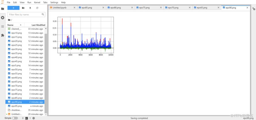
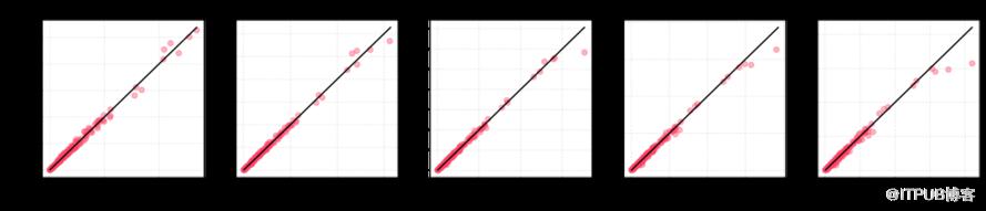
图4横轴表示文献的真实被引量,纵轴表示文献的预测被引量,距离黑线越近说明预测结果越好。可以看出随着预测长度增加,预测偏差逐渐变大了。
6.待讨论的问题
2021年北航团队将Transformer模型进行了改进,在文献 Informer: Beyond Efficient Transformer for Long Sequence Time-Series Forecasting 提出了更适合进行时间序列预测 Informer 模型,获得了AAAI 2021 的 Best Paper, 后面笔者也会抽时间学习~
参考文献
[1] Vaswani A, Shazeer N, Parmar N, et al. Attention is all you need[J]. arXiv preprint arXiv:1706.03762, 2017.
[2] Oliver Guhr. Transformer Time Series Prediction.
附件
完整代码及部分数据请参考:链接:https://pan.baidu.com/s/1-I1c8UOXvkfAqiQLcymfDA 提取码:1234 想要和作者交流想法,可以加作者微信号:wkh18765699194

图神经网络(04)-[彩蛋和实战] 基于Graph的传统机器学习方法
添加助手微信加入微信交流群或者QQ交流群:



原文作者:ChallengeHub;如有侵权,请联系管理员删除。

